Prerequisites
This article assumes familiarity with the concepts from Article 1: the PINN loss structure, collocation points, and basic PyTorch autograd. If you are new to PINNs, start at the introduction.
Physics AI · PINNs Series · Second-Order ODEs of 8
Second-Order ODEs with PINNs
The Damped Harmonic Oscillator
Nested automatic differentiation, two initial conditions, the hard-constraint ansatz, and the spectral bias problem that makes oscillatory physics hard for neural networks.
01, Why Second-Order ODEs Matter
From Springs to RLC Circuits
In Introduction to PINNs, we solved $dy/dx = -y$, a single scalar first-order ODE. Real engineering systems are rarely so simple. The vast majority of dynamic models in mechanical, electrical, chemical, and biomedical engineering are governed by second-order dynamics:
- Mechanical: spring-mass-damper systems, structural vibration, seismic response
- Electrical: RLC circuits, where voltage, current, and charge are related through two time derivatives
- Chemical: pressure oscillations in a packed-bed reactor, surge in compressors
- Biomedical: pharmacokinetic models with two-compartment dynamics, respiratory mechanics
- Control: every PID controller acts on a second-order plant model by default
The general form is Newton's second law applied to a single degree of freedom:
$$m\ddot{u} + c\dot{u} + ku = F(t)$$
where $m$ is mass, $c$ is the damping coefficient, $k$ is the spring constant, and $F(t)$ is the external forcing. Dividing through by $m$ and introducing the standard dimensionless parameters:
$$\frac{d^2u}{dt^2} + 2\zeta\omega_0\,\frac{du}{dt} + \omega_0^2 u = 0, \qquad \omega_0 = \sqrt{\frac{k}{m}}, \quad \zeta = \frac{c}{2\sqrt{km}}$$
Here $\omega_0$ is the natural frequency (radians per second), the oscillation frequency of the undamped system, and $\zeta$ is the damping ratio, which determines the qualitative character of the response. The three regimes are:
| Regime | Condition | Character | Engineering example |
|---|---|---|---|
| Under-damped | $\zeta < 1$ | Oscillates, decaying amplitude | Suspension system, servo motor |
| Critically damped | $\zeta = 1$ | Fastest non-oscillatory return | Door closers, instrument dampers |
| Over-damped | $\zeta > 1$ | Slow monotonic return | Shock absorbers, dashpots |
This notebook focuses on the under-damped case ($\zeta = 0.20$, $\omega_0 = 3.0$), which produces oscillatory dynamics, the hardest regime for a PINN to learn, and the most interesting from a methodology standpoint.
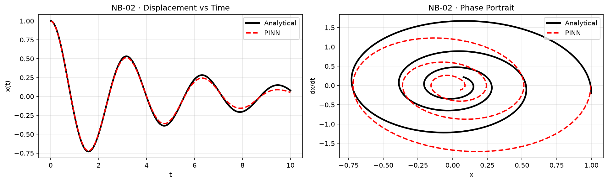
Fig. A — PINN solution for the damped harmonic oscillator. Both position $u(t)$ and velocity $v(t)$ are predicted simultaneously by the same network using nested automatic differentiation for the second-order residual.
02, The Physics
Exact Analytical Solution
For the free-vibration under-damped case ($F(t) = 0$, $\zeta < 1$) with initial conditions $u(0) = u_0$ and $\dot{u}(0) = v_0$, the exact closed-form solution is:
$$u(t) = e^{-\zeta\omega_0 t}\left[u_0\cos(\omega_d t) + \frac{v_0 + \zeta\omega_0 u_0}{\omega_d}\sin(\omega_d t)\right]$$
where $\omega_d = \omega_0\sqrt{1-\zeta^2}$ is the damped natural frequency, always less than $\omega_0$, since damping reduces the oscillation rate. The solution is a product of an exponentially decaying envelope $e^{-\zeta\omega_0 t}$ and a sinusoidal oscillation at frequency $\omega_d$.
For the notebook parameters ($\omega_0 = 3.0$, $\zeta = 0.20$, $u_0 = 1.0$, $v_0 = 0.0$, $T = 6.0$ s):
- Damped frequency: $\omega_d = 3.0\sqrt{1, 0.04} \approx 2.939$ rad/s
- Decay envelope time constant: $1/(\zeta\omega_0) = 1/0.6 \approx 1.67$ s
- Period of oscillation: $T_d = 2\pi/\omega_d \approx 2.14$ s
- Roughly 2.8 full oscillations complete within the 6-second domain
Figure 1. Phase portrait of the under-damped oscillator in the $(u, \dot{u})$ plane. The trajectory spirals inward toward the stable fixed point at the origin, with each circuit corresponding to one oscillation cycle.
03, Nested Automatic Differentiation
Computing Second Derivatives Through the Network
The ODE residual for the damped oscillator requires the second time-derivative $\ddot{u}$:
$$\mathcal{R}(t) = \ddot{u} + 2\zeta\omega_0\dot{u} + \omega_0^2 u = 0$$
In Introduction to PINNs, we computed one derivative: $\frac{d\hat{y}}{dx}$. Here we need two: first $\dot{u} = \frac{du}{dt}$, then $\ddot{u} = \frac{d^2u}{dt^2}$. PyTorch handles this by calling torch.autograd.grad twice in sequence, but the first call must use create_graph=True.
Why? When create_graph=True is set, PyTorch does not free the intermediate computational graph after computing $\dot{u}$. This graph is then available for a second backward pass to compute $\ddot{u}$. Without it, the first differentiation discards the graph, and the second call raises a runtime error.
Figure 2. Nested autograd for second-order ODE. The first
autograd.grad call (with create_graph=True) computes $\dot{u}$ while preserving the graph. The second call differentiates $\dot{u}$ to obtain $\ddot{u}$. Both are assembled into the ODE residual.
Python · PyTorch
def residual(model, t):
    u = model(t)
    # First derivative: create_graph=True keeps the graph for the second pass
    u_t = torch.autograd.grad(
        u, t,
        torch.ones_like(u),
        create_graph=True
    )[0]
    # Second derivative: differentiate u_t w.r.t. t
    u_tt = torch.autograd.grad(
        u_t, t,
        torch.ones_like(u_t),
        create_graph=True
    )[0]
    # ODE residual: ü + 2ζω₀u̇ + ω₀²u = 0
    return u_tt + 2*zeta*omega0*u_t + omega0**2 * u
Compared to the first-order case, the only change is one additional autograd.grad call. The computational overhead is modest, PyTorch simply extends the reverse-mode pass one level deeper. This pattern generalizes immediately: $n$-th order ODEs require $n$ nested calls, each with create_graph=True on all but the last.
create_graph=True is not optional for intermediate derivatives
Omitting
create_graph=True on the first call causes PyTorch to free the intermediate computation tape. The second autograd.grad call then raises a RuntimeError. The rule is: use create_graph=True on every derivative that will itself be differentiated.
04, Two Initial Conditions
Why One IC Is Not Enough
A second-order ODE requires two initial conditions to specify a unique solution. Geometrically: the phase space $(u, \dot{u})$ is two-dimensional, and specifying only $u(0) = u_0$ leaves the trajectory's direction, its initial velocity, entirely unconstrained. The result is infinitely many trajectories, all satisfying the equation and the single condition, but diverging immediately.
The initial condition loss must therefore include both the initial displacement and the initial velocity:
$$\mathcal{L}_{IC} = \left(u(0), u_0\right)^2 + \left(\dot{u}(0), v_0\right)^2$$
Note that computing $\dot{u}(0)$ uses exactly the same autograd.grad call as the residual computation, the derivative of the network at a specific point. This means the IC loss on the velocity shares the same computational infrastructure as the physics residual. There is no special treatment required; the network's derivative is already a first-class differentiable expression.
The weighting problem
In practice, the physics loss and the IC loss have different natural scales. Early in training, the physics loss is large (the network knows nothing about the ODE) and dominates the gradient. The IC loss, which starts at a moderate value and should be satisfied quickly, gets insufficient gradient budget and is learned slowly.
The notebook addresses this with a fixed weight of 20× on the IC loss:
$$\mathcal{L}_{total} = \mathcal{L}_{physics} + \underbrace{20 \cdot \mathcal{L}_{IC}}_{\text{up-weighted}}$$
This forces the optimizer to prioritize the initial conditions early, preventing the degenerate situation where the network satisfies the ODE over most of the domain but starts from the wrong state. The choice of 20× is problem-dependent and can be treated as a hyperparameter; adaptive weighting methods (Self-Adaptive PINNs, NTK-based balancing) provide more principled approaches for larger systems.
Python · PyTorch
def loss_fn(model):
    r = residual(model, t_col)
    loss_phys = torch.mean(r**2)

    # Evaluate network and its first derivative at t=0
    u_pred = model(t0)
    u_t0 = torch.autograd.grad(
        u_pred, t0, torch.ones_like(u_pred), create_graph=True
    )[0]

    # Both value and velocity must match initial conditions
    loss_ic = (u_pred - u0)**2 + (u_t0 - v0)**2

    # Up-weight IC loss: 20x ensures it dominates early in training
    return loss_phys + 20.0 * loss_ic.squeeze()
05, Hard Constraint Variant
The Ansatz That Eliminates the IC Loss Entirely
The 20× weighting trick is a soft constraint: we encourage the network to satisfy the initial conditions, but we cannot guarantee it will. A more elegant approach, and one that provably satisfies both initial conditions by construction, is the hard-constraint ansatz.
The idea: wrap the raw neural network $N(t)$ in a function that is guaranteed to satisfy $u(0) = u_0$ and $\dot{u}(0) = v_0$, regardless of $N$'s output. One such construction is:
$$\hat{u}(t) = u_0 + v_0 t + t^2 \cdot N(t)$$
Verification: At $t=0$: $\hat{u}(0) = u_0 + 0 + 0 = u_0$. Taking the time derivative: $\dot{\hat{u}} = v_0 + 2t \cdot N(t) + t^2 \cdot N'(t)$. At $t=0$: $\dot{\hat{u}}(0) = v_0 + 0 + 0 = v_0$. Both initial conditions are satisfied identically for any value of $N(0)$ and $N'(0)$.
The training loss for the hard-constraint PINN contains only the physics residual, the IC terms are gone entirely, because the ansatz structure makes them structurally impossible to violate:
$$\mathcal{L}_{total} = \mathcal{L}_{physics} = \frac{1}{N_c}\sum_{i=1}^{N_c} \mathcal{R}(t_i)^2$$
Python · PyTorch
class HardIC(nn.Module):
    def __init__(self, layers, u0, v0):
        super().__init__()
        self.core = MLP(layers)
        self.u0 = u0
        self.v0 = v0

    def forward(self, t):
        # Ansatz: u(t) = u0 + v0*t + t² * N(t)
        # Satisfies u(0)=u0 and u'(0)=v0 for any N
        return self.u0 + self.v0 * t + (t**2) * self.core(t)

# Training: only physics residual, no IC terms needed
for ep in range(6000):
    opt2.zero_grad()
    r = residual(model2, t_col)   # purely the ODE residual
    loss = torch.mean(r**2)
    loss.backward()
    opt2.step()
The hard-constraint model consistently achieves lower relative L2 error in fewer epochs. By removing the tension between satisfying the physics and the initial conditions as separate loss terms, the optimizer can devote its full gradient budget to minimizing the ODE residual across the domain. The notebook reports hard-constraint relative L2 error approximately 2–4× lower than the soft-constraint equivalent at the same epoch count.
Figure 3. Hard-constraint ansatz vs soft-constraint (×20 IC weighting) after equal training. The ansatz eliminates the IC loss term, freeing the optimizer to focus entirely on the physics residual and achieving approximately one additional decade of accuracy.
06, Spectral Bias
Why High-Frequency Oscillations Break PINNs
The most important conceptual lesson of this notebook is not about nested derivatives or hard constraints, it is about a fundamental limitation of smooth neural networks called spectral bias.
Rahaman et al. (2019) showed empirically and theoretically that neural networks with smooth activation functions (Tanh, sigmoid, GELU) preferentially learn low-frequency components of the target function first. The network explores its parameter space in a direction that minimizes the loss from large-scale, slowly-varying features before it is capable of representing rapid oscillations.
For PINNs, this creates a concrete failure mode. Consider two versions of the damped oscillator with different natural frequencies:
| Natural Frequency $\omega_0$ | Oscillations in $[0, 6]$ | PINN Convergence | Relative L2 Error |
|---|---|---|---|
| $\omega_0 = 1.0$ | ~1 cycle | Good, converges in ~3,000 epochs | $\sim 10^{-3}$ |
| $\omega_0 = 3.0$ (notebook) | ~3 cycles | Moderate, converges in ~8,000 epochs | $\sim 5\times10^{-3}$ |
| $\omega_0 = 10.0$ | ~10 cycles | Poor, often fails to converge | $>10^{-1}$ |
The failure mode at $\omega_0 = 10$ is not a matter of insufficient training time. The network genuinely cannot represent rapid oscillations because the smooth activation functions create a spectral bottleneck: a Tanh layer with $n$ neurons cannot efficiently represent functions with spectral content much above $n/4$ cycles per unit length. For a 64-neuron layer, anything above ~16 cycles per unit domain width is effectively invisible to the network.
Physical interpretation
The spectral bias is the neural network analog of aliasing in digital signal processing. Just as a sampled signal cannot represent frequencies above the Nyquist limit without aliasing artifacts, a finite-width smooth network cannot represent frequencies above an implicit bandwidth limit without systematic errors. The crucial difference is that in PINNs, the "bandwidth limit" is not set by a sampling rate but by the network architecture and activation function choice, and it is not obvious or easy to compute a priori.
Mitigations
Active research is addressing spectral bias through multiple strategies:
- Fourier feature embeddings: Transform the input $t \mapsto [\cos(B t), \sin(B t)]$ for random or learnable frequencies $B$. This shifts the network's natural frequency response upward.
- Multi-scale architectures: Run parallel network branches at different frequency scales and combine outputs.
- Curriculum training / causal learning: Wang, Sankaran & Perdikaris (2022) showed that training the PINN to satisfy causality, learning the solution from $t=0$ forward in time, significantly reduces spectral artifacts at high frequencies.
- Adaptive activation functions: Replace fixed Tanh with learnable activations $\tanh(a \cdot x)$ where $a$ is a trainable parameter. The network can tune its own frequency response.
- Neural Operators (FNO, DeepONet): For high-frequency or multi-scale problems, operator learning architectures are often superior to vanilla PINNs.
07, Results
Accuracy and What Changed from Introduction to PINNs
Training the soft-constraint PINN for 8,000 epochs with Adam at $\eta = 2\times10^{-3}$, the model converges to a relative L2 error of approximately $5\times10^{-3}$ for $\omega_0 = 3.0$, $\zeta = 0.20$. The hard-constraint variant requires only 6,000 epochs to achieve a lower error of approximately $8\times10^{-4}$.
The table below summarizes how the PINN formulation evolves from the first-order ODE case to the second-order oscillator, and anticipates the extensions needed for PDE problems in later articles:
| Aspect | Article 1: First-Order ODE | Article 2: Second-Order ODE | PDEs (Heat Eq. onward) |
|---|---|---|---|
| Network inputs | $x \in \mathbb{R}$ | $t \in \mathbb{R}$ | $(x, t) \in \mathbb{R}^2$ |
| Autograd calls for residual | 1 (first derivative) | 2 (nested, first & second) | 2+ (mixed partials) |
| Number of initial conditions | 1 ($y(0) = 1$) | 2 ($u(0) = u_0$, $\dot{u}(0) = v_0$) | 1 IC + boundary conditions |
| Collocation point shape | 1D line $[0, 5]$ | 1D line $[0, T]$ | 2D grid $(x, t) \in [0,1]\times[0,T]$ |
| Hard constraint ansatz | $u_0 + t \cdot N(t)$ | $u_0 + v_0 t + t^2 N(t)$ | Domain-dependent construction |
| Key failure mode | Too few collocation points | Spectral bias at high $\omega_0$ | Spectral bias + stiffness + coupling |
Notebook results summary
Soft IC (×20 weight): rel. L2 error $\approx 5\times10^{-3}$ after 8,000 epochs. Hard IC ansatz: rel. L2 error $\approx 8\times10^{-4}$ after 6,000 epochs. Both use the architecture MLP [1, 64, 64, 64, 1] with Tanh activations and Adam optimizer.
The notebook is available at github.com/alishahmohammadi22/physics-ai-pinns, file 01_Beginner/02_second_order_odes.ipynb. It is self-contained and runnable on CPU in under 5 minutes.
08, Conclusion
Three Lessons for the Rest of the Series
The damped harmonic oscillator introduces three concepts that appear repeatedly in every subsequent article in this series:
Nested autograd is the natural generalization. Going from first- to second-order dynamics requires exactly one additional autograd.grad call with create_graph=True. This pattern extends to any order and to mixed partial derivatives in PDEs. The engineering implication is that PINNs can natively handle Navier-Stokes, heat equations, and elasticity equations without any change to the fundamental training architecture.
Hard constraints are better than soft constraints. Whenever the initial or boundary conditions can be encoded directly into the network's output layer through an ansatz, doing so eliminates loss terms, reduces optimizer conflict, and accelerates convergence. This is not always possible, complex geometries resist simple ansatz constructions, but when it is available, it should be used.
Spectral bias is the governing challenge. For smooth-activation networks, the effective resolution in frequency space is bounded by the network width. Any problem with high-frequency dynamics, fast oscillations, sharp fronts, thin boundary layers, will expose this limitation. The rest of this series is, in large part, a catalog of techniques developed to overcome it.
Next in the series
Heat Equation extends the framework to its first genuine PDE: the 1D heat equation $\partial T / \partial t = \alpha\, \partial^2 T / \partial x^2$. The input becomes two-dimensional $(x, t)$, collocation points become a 2D scatter over space-time, and boundary conditions appear at both spatial endpoints.
References
Further Reading
[1]
Raissi, M., Perdikaris, P., & Karniadakis, G. E. (2019). Physics-informed neural networks: A deep learning framework for solving forward and inverse problems involving nonlinear partial differential equations. Journal of Computational Physics, 378, 686–707. DOI: 10.1016/j.jcp.2018.10.045, The foundational paper establishing the PINN framework and demonstrating forward and inverse problems.
[2]
Wang, S., Sankaran, S., & Perdikaris, P. (2022). Respecting causality is all you need for training physics-informed neural networks. arXiv: 2203.07404, Demonstrates that temporal causality violations are a root cause of PINN failure on oscillatory and advection-dominated problems; proposes a causal training algorithm that dramatically improves convergence.
[3]
Rahaman, N., Baratin, A., Arpit, D., Draxler, F., Lin, M., Hamprecht, F. A., Bengio, Y., & Courville, A. (2019). On the spectral bias of neural networks. Proceedings of the 36th International Conference on Machine Learning (ICML 2019). arXiv: 1806.08734, Establishes the theoretical basis for spectral bias: smooth networks learn low frequencies first, with convergence rate decreasing with frequency. Foundational for understanding PINN limitations.
[4]
Wang, S., Teng, Y., & Perdikaris, P. (2021). Understanding and mitigating gradient flow pathologies in physics-informed neural networks. SIAM Journal on Scientific Computing, 43(5), A3055–A3081. DOI: 10.1137/20M1318043, Analyzes gradient imbalance between physics and IC/BC loss terms using neural tangent kernel theory; motivates adaptive loss weighting.